Postgres vs. Oracle access paths VII – Bitmap Index Scan

By Franck Pachot

.
In the previous post we have seen the Index Scan, where a where clause condition uses the index structure to find rows and then fetches remaining columns from the table. The case was an optimal one where the correlation/clustering factor was good. Now I’ll do the opposite: the worst clustering factor.

Index with good correlation / clustering factor

The table used in the previous post was created with:

create table demo1 as select generate_series n , 1 a , lpad('x',1000,'x') x from generate_series(1,10000);
create unique index demo1_n on demo1(n);

Because the index order (on the increasing number coming from generate_series) matches the order of the rows inserted, we had a good probability that an index scan will find rows in the same block as the previous index entry. As we have seen, this optimal case is considered by the optimizer (cost evaluated on the number of blocks rather than on the number of rows) as well as by the execution engine (reads processed as sequential reads allowing read-ahead and prefetching).

Basically, both Oracle and Postgres estimates, and reads, about 150 blocks to read 1000 rows (over the 1500 pages table storing 10000 rows).

147 in Postgres:

explain (analyze,verbose,costs,buffers) select  a from demo1  where n<=1000 ;
                                                          QUERY PLAN
------------------------------------------------------------------------------------------------------------------------------
 Index Scan using demo1_n on public.demo1  (cost=0.29..175.78 rows=1000 width=4) (actual time=0.029..0.780 rows=1000 loops=1)
   Output: a
   Index Cond: (demo1.n <= 1000)
   Buffers: shared hit=147
 Planning time: 1.019 ms
 Execution time: 0.884 ms

148 in Oracle:

select /*+  */  a from demo1  where n<=1000
----------------------------------------------------------------------------------------------------------------------
| Id  | Operation                           | Name    | Starts | E-Rows | Cost (%CPU)| A-Rows |   A-Time   | Buffers |
----------------------------------------------------------------------------------------------------------------------
|   0 | SELECT STATEMENT                    |         |      1 |        |   147 (100)|   1000 |00:00:00.01 |     148 |
|   1 |  TABLE ACCESS BY INDEX ROWID BATCHED| DEMO1   |      1 |   1000 |   147   (0)|   1000 |00:00:00.01 |     148 |
|*  2 |   INDEX RANGE SCAN                  | DEMO1_N |      1 |   1000 |     4   (0)|   1000 |00:00:00.01 |       4 |
----------------------------------------------------------------------------------------------------------------------
Predicate Information (identified by operation id):
---------------------------------------------------
   2 - access("N"<=1000)

This is optimal, but not always achievable because:

• Not all indexes can have a good correlation as there’s only one physical order of the table
• The physical order in the table depends on the insert order (and updates in Postgres as they are processed as delete+insert)

Index with bad correlation / clustering factor

I’m creating a second table DEMO2 similar to DEMO1 but with a different physical order where 1000 consecutive index entries are scattered throughout the whole table.

In Postgres:

create table demo2 as select * from demo1 order by mod(n,1000);
create unique index demo2_n on demo2(n);
vacuum analyze demo2;

In Postgres, the correlation is measured for each columns and the statistics stores it as a factor between 0 (values scattered though the table) and 1 (values clustered):

 select tablename,attname, correlation from pg_stats where tablename like 'demo_' and attname='n';
 
 tablename | attname | correlation
-----------+---------+-------------
 demo1     | n       |           1
 demo2     | n       |   0.0992811

In Oracle:

create table demo2 as select * from demo1 order by mod(n,1000);
create unique index demo2_n on demo2(n);
exec dbms_stats.gather_table_stats(user,'demo2');

In Oracle, the correlation is measured for each index and the statistics stores it as the number of table blocks to read when we scan the index entries in order. This is called ‘clustering factor’ and is a value between the number of index entries (good clustering) and the number of table blocks (bad clustering):

select table_name,index_name,clustering_factor from dba_ind_statistics where table_name like 'DEMO_' and index_name like 'DEMO__N';
 
TABLE_NAME INDEX_NAME CLUSTERING_FACTOR
---------- ---------- -----------------
DEMO1      DEMO1_N                 1429
DEMO2      DEMO2_N                 9968

My table has 10000 rows indexed and 1429 table blocks.

Oracle

I’ll run the same query as above, but now on DEMO2. And in order to compare, I force the same plan with the INDEX() hint:

PLAN_TABLE_OUTPUT
------------------------------------------------------------------------------------------------------------------------------------------------------
SQL_ID  0t6t26pvw763m, child number 0
-------------------------------------
select /*+ index(demo2) */  a from demo2  where n<=1000
----------------------------------------------------------------------------------------------------------------------
| Id  | Operation                           | Name    | Starts | E-Rows | Cost (%CPU)| A-Rows |   A-Time   | Buffers |
----------------------------------------------------------------------------------------------------------------------
|   0 | SELECT STATEMENT                    |         |      1 |        |  1001 (100)|   1000 |00:00:00.01 |    1000 |
|   1 |  TABLE ACCESS BY INDEX ROWID BATCHED| DEMO2   |      1 |   1000 |  1001   (0)|   1000 |00:00:00.01 |    1000 |
|*  2 |   INDEX RANGE SCAN                  | DEMO2_N |      1 |   1000 |     4   (0)|   1000 |00:00:00.01 |       4 |
----------------------------------------------------------------------------------------------------------------------
Predicate Information (identified by operation id):
---------------------------------------------------
   2 - access("N"<=1000)
Column Projection Information (identified by operation id):
-----------------------------------------------------------
   1 - "A"[NUMBER,22]
   2 - "DEMO2".ROWID[ROWID,10]

The cost is higher: estimates 1000 random reads, one for each row, and the actual number of block reads show the same: 1000 buffers. This is the cost of bad clustering factor: read as many blocks as the index entries. This is obviously not efficient because a block contains several rows, and we read the whole to get only one row.

The optimizer is aware of that and does not choose this execution plan. Without hints, a full tablespace is chosen:

PLAN_TABLE_OUTPUT
------------------------------------------------------------------------------------------------------------------------------------------------------
SQL_ID  4y654kzqv9dx1, child number 0
-------------------------------------
select /*+  */  a from demo2  where n<=1000
--------------------------------------------------------------------------------------------------
| Id  | Operation         | Name  | Starts | E-Rows | Cost (%CPU)| A-Rows |   A-Time   | Buffers |
--------------------------------------------------------------------------------------------------
|   0 | SELECT STATEMENT  |       |      1 |        |   397 (100)|   1000 |00:00:00.01 |    1450 |
|*  1 |  TABLE ACCESS FULL| DEMO2 |      1 |   1000 |   397   (0)|   1000 |00:00:00.01 |    1450 |
--------------------------------------------------------------------------------------------------
Predicate Information (identified by operation id):
---------------------------------------------------
   1 - filter("N"<=1000)
Column Projection Information (identified by operation id):
-----------------------------------------------------------
   1 - "A"[NUMBER,22]

More buffers to read (1450 instead of 1000) but read in multi-block sequential read, for which the cost is lower (the 0.278 factor we have seen in first post).

Postgres

As I did for Oracle, I’m running the same query, now on DEMO2. And in order to compare, I force the same plan with the IndexScan() hint:

/*+ IndexScan(demo2) */
explain (analyze,verbose,costs,buffers) select  a from demo2  where n<=1000 ;
                                                          QUERY PLAN
-------------------------------------------------------------------------------------------------------------------------------
 Index Scan using demo2_n on public.demo2  (cost=0.29..2966.01 rows=1000 width=4) (actual time=0.018..1.562 rows=1000 loops=1)
   Output: a
   Index Cond: (demo2.n <= 1000)
   Buffers: shared hit=923
 Planning time: 0.394 ms
 Execution time: 1.635 ms

The same thing as we have seen in Oracle: nearly one new block for each index entry. The Index Scan has read 923 buffers.

As we have seen previously, the cost estimation includes:

• We have 1000 index entries to process, estimated at cost=5 (cpu_index_tuple_cost=0.005)
• We have 1000 result rows to process, estimated at cost=10 (cpu_tuple_cost=0.01)
• We have evaluated 1000 ‘is not null’ conditions, estimated at cost=2.5 (cpu_operator_cost=0.0025)
• We about 116 operation for the startup cost so that cost=0.29 (cpu_operator_cost=0.0025)

Then the CPU cost is cost=0.29+2.5+18+5=25.79 and remains cost=2966.01-25.79=2940.22 for I/O. As they are random reads, except the first one, we know that the query planner estimated them to (2940.22-1)/4=734.805

Cache hit estimation

The number of estimated rows calculated above (734.805) looks weird: under estimated, and not an integer. This is because there’s another parameter used by the query planner:

show effective_cache_size;
 effective_cache_size
----------------------
 4GB

The optimizer knows the size of the buffer cache and then estimates that not all buffer gets will be physical reads. Let’s run the same as before but estimating the buffer cache to one block only:

begin transaction;
BEGIN
set local effective_cache_size=1;
SET
/*+ IndexScan(demo2) */
explain (analyze,verbose,costs,buffers) select  a from demo2  where n<=1000 ;
                                                          QUERY PLAN
-------------------------------------------------------------------------------------------------------------------------------
 Index Scan using demo2_n on public.demo2  (cost=0.29..3991.80 rows=1000 width=4) (actual time=0.024..1.884 rows=1000 loops=1)
   Output: a
   Index Cond: (demo2.n <= 1000)
   Buffers: shared hit=923
 Planning time: 0.630 ms
 Execution time: 2.002 ms

The estimated cost here is much higher: cost=3991.80 which, given the random_page_cost=4, estimates 990 rows.

This is interesting. It is always a challenge for the optimizer to estimate how many buffer reads are a cache hit in order to decrease the estimation of physical reads. Oracle had some attempts with _optimizer_cache_stats and optimizer_index_caching. Here it seems that Postgres uses a factor which depends on the size of the buffer cache (and the filesystem cache). This will deserve a new blog post, but here is already an idea. I’ve increased effective_cache_size from 1 page (8k) to 10000 pages (my table is 1500 pages) and got the following:

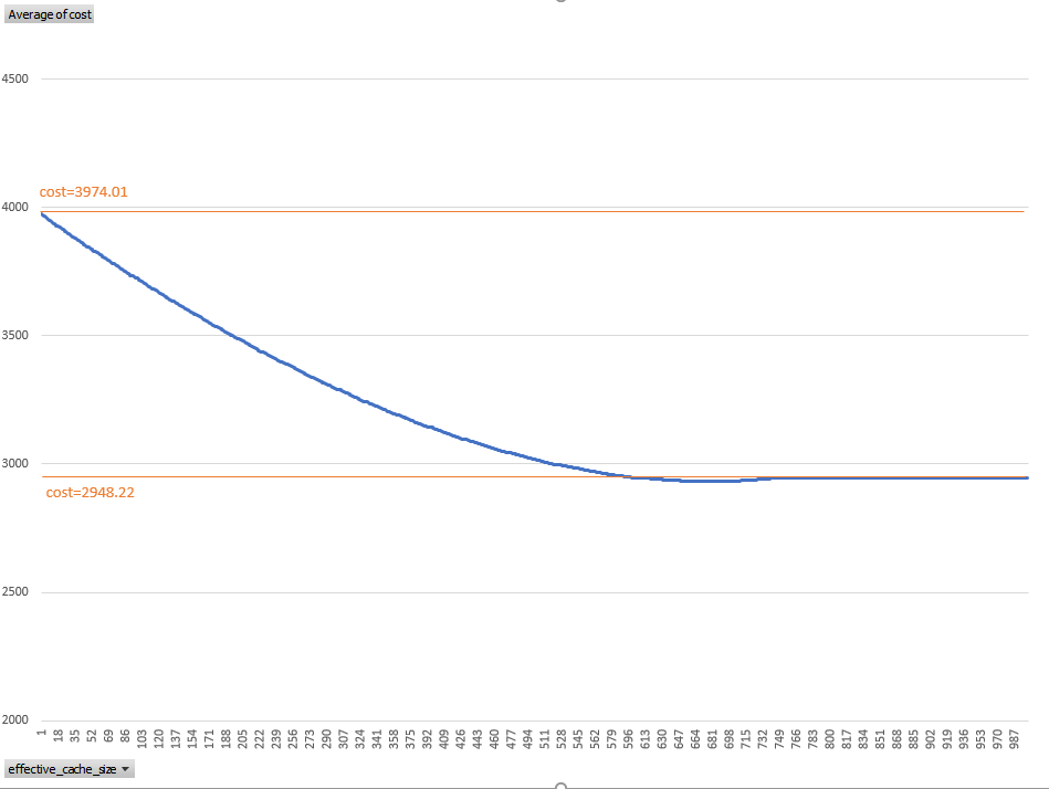
With no buffer cache, the cost=4000 which is the random_page_cost for the 1000 blocks I have to read.
When the buffer cache has enough space for about 40% of the table, then the cost is estimated to 75% of the no-cache one.

Of course, because Postgres is Open Source, all formulas are public. Look for index_pages_fetched in costsize.c

When clustering factor is bad, Oracle prefers to do a full table scan. In the same idea, Postgres has a lower estimated cost for Seq Scan (cost=1554) rather than Index Scan (cost=3991.80):

/*+ SeqScan(demo2) */
explain (analyze,verbose,costs,buffers) select  a from demo2  where n<=1000 ;
                                                  QUERY PLAN
---------------------------------------------------------------------------------------------------------------
 Seq Scan on public.demo2  (cost=0.00..1554.00 rows=1000 width=4) (actual time=0.025..3.811 rows=1000 loops=1)
   Output: a
   Filter: (demo2.n <= 1000)
   Rows Removed by Filter: 9000
   Buffers: shared hit=1429
 Planning time: 0.716 ms
 Execution time: 3.922 ms

The cost is calculated from 1429 sequential reads (at seq_page_cost=1), 10000 tuples (at cpu_tuple_cost=0.01) and 10000 ‘greater than’ operators (at cpu_operator_cost=0:0.0025) which sums to cost=1554.

Bitmap Heap Scan

However, without any hint, the query planner uses an access path which is even cheaper:

explain (analyze,verbose,costs,buffers) select  a from demo2  where n<=1000 ;
                                                       QUERY PLAN
------------------------------------------------------------------------------------------------------------------------
 Bitmap Heap Scan on public.demo2  (cost=20.04..1395.75 rows=1000 width=4) (actual time=0.210..1.942 rows=1000 loops=1)
   Output: a
   Heap Blocks: exact=919
   Recheck Cond: (demo2.n <= 1000)
   < Bitmap Index Scan on demo2_n  (cost=0.00..19.79 rows=1000 width=0) (actual time=0.122..0.122 rows=1000 loops=1)
         Index Cond: (demo2.n <= 1000)
         Buffers: shared hit=4
 Planning time: 0.639 ms
 Execution time: 2.027 ms

The idea here is to avoid to re-visit a page that has already been visited from another index entry, as Index Scan does. But also avoid to read all pages. This is why we see two steps: one to scan the index, and the other one to scan the table, using the index scan result as a list of pages to read.

The Bitmap Index Scan is a range scan, reading 10% of the index (because we have 10000 index entries and the range predicate is “<1000). The index has 30 pages, then the cost is estimated to 3 random reads (at random_page_cost=4) with cost=12. We add 1000 index entries (cpu_index_tuple_cost=0.005) at cost=5 and 1000 '<1000' operators (cpu_operator_cost=0.0025) at cost=2. There is an initial startup cost at 116 operations, as we have seen for all index accesses whith cost=2.79 and then the total cost of Bitmap Index Scan is cost=19.79.

The output of this operation is a bitmap which will be used to know which table pages to read.

This read of the table is the Bitmap Heap Scan step. The initial cost for it is the total cost of the previous step: before returning any rows, the Bitmap Heap Scan cannot start until the bitmap is built. In addition to this initial cost, the major cost components are page reads. I have at least 10% of the table to read if all my 1000 rows were clustered, on this 1429 pages, 10000 rows table. In this case, those pages may be sequential or not. But with bad clustering factor, I may have 1429 pages to read if the 1000 rows are scattered on all the table. In this case, those pages are sequential because I read all of them. then, the query planner has two estimations to do: the number of pages (from the correlation factor) and the proportion of contiguous ones, where multiple pages can be read with only one lseek().

In my case, I’ve ‘explain plan’ with all query planner constants set to 0 except seq_page_cost=1 and the cost was:

set local seq_page_cost=1;set local random_page_cost=0;set local cpu_tuple_cost=0;set local cpu_index_tuple_cost=0;set local cpu_operator_cost=0;
...
/*+ BitmapScan(demo2) */ explain (analyze,verbose,costs,buffers) select  a from demo2  where n  Bitmap Index Scan on demo2_n  (cost=0.00..0.00 rows=1000 width=0) (actual time=0.129..0.129 rows=1000 loops=1)
...

The query planner estimated 533.59 sequential reads, which is about 37% of my table.

Then the same setting only the randdom read cost:

set local seq_page_cost=0;set local random_page_cost=4;set local cpu_tuple_cost=0;set local cpu_index_tuple_cost=0;set local cpu_operator_cost=0;
...
/*+ BitmapScan(demo2) */ explain (analyze,verbose,costs,buffers) select  a from demo2  where n  Bitmap Index Scan on demo2_n  (cost=0.00..12.00 rows=1000 width=0) (actual time=0.174..0.174 rows=1000 loops=1)
...

The query planner estimated (841.62-12)/4=207 random reads, which is about 14% of my table.

Those Bitmap Heap Scan adds 1363.23 to the cost of Bitmap Index Scan.
The remaining to get the total cost=1395.75 is 12.73 and there is obviously 1000 tuples at cpu_tuple_cost=0.01 which counts for cost=10
Then remains cost=2.73 and this is approximately 2.73/0.0025=1092 cpu operator cost. If you look at the plan above, you can see the ‘n<=1000' condition in the Bitmap Index Scan index condition:

         Index Cond: (demo2.n <= 1000)

This creates a bitmap of pages and rows that verify the predicate. But this bitmap may be large for many rows, and then become less efficient. Postres optimizes that by creating a smaller bitmap with false positives: mentioning the whole page when many rows are there. This reduces the bitmap (no detail about which rows within the block) but then the predicate must be checked again to remove false positives. When can see that in the recheck condition:

   Recheck Cond: (demo2.n <= 1000)

And this explains the additional cpu cost for 1000 cpu_operator_cost

So what?

This post shows the most difficult part of the optimizer access path.

When you want most of the rows, the choice is easy: Seq Scan. When you want few rows from a correlated index: Index Scan. But lot of queries are in the middle, such as this example, querying 10% of rows scattered within the table.

This is where the different RDBMS had to implement different optimizations, especially at the time where random reads had to seek with big latencies. You find same concepts (prefetching, bitmap, batching) but used differently. Oracle uses bitmaps (stored or on the fly) mainly when they can be combined. We have seen that Postgres can choose bitmap access even when there is one, just to filter and sort the pages to read. Oracle does something similar with the BY INDEX ROWID BATCHED, except that it works on a vector to filter and sort the ROWIDs needed by the next fetch. In all cases, this defeats what we have seen with ORDER BY queries three posts ago, as this batching/two-steps optimization changes the logical order of the index to the physical order of the table.

In the next post, I’ll add some condition on this indexed columns because besides the index condition (or access predicate) I want to filter out most rows before going to the table.